Cloud Optimized ERA5

Cloud Optimized ERA5#

In their public dataset program, Google’s Cloud Storage provides a variety of public datasets that can be accessed by the community. Google pays for the hosting of these datasets.

One of these datasets is an “Analysis-Ready, Cloud Optimized” (ARCO) ERA5 dataset. This is based on the European Centre for Medium-Range Weather Forecasts (ECMWF) Atmospheric Reanalysis product, a very commonly used dataset for world-wide historical meteorological parameters ranging from 1940 to now.

Accessing the dataset#

This dataset uses Zarr to make access very easy.

You might need to install the following dependencies still:

%pip install xarray matplotlib zarr gcsfs

Now we can open the Zarr store with the following code (copied from the ARCO-ERA5 github page).

import xarray

ds = xarray.open_zarr(
    'gs://gcp-public-data-arco-era5/ar/full_37-1h-0p25deg-chunk-1.zarr-v3',
    chunks=None,
    storage_options=dict(token='anon'),
)
ar_full_37_1h = ds.sel(time=slice(ds.attrs['valid_time_start'], ds.attrs['valid_time_stop']))

How to use xarray with Zarr stores#

The data is opened as an xarray “Dataset”. This dataset holds all variables and their associated dimensions and coordinates. As you can see, there are 273 variables contained in this dataset:

ar_full_37_1h

<xarray.Dataset> Size: 2PB
Dimensions:                                                          (
                                                                      time: 740712,
                                                                      latitude: 721,
                                                                      longitude: 1440,
                                                                      level: 37)
Coordinates:
  * latitude                                                         (latitude) float32 3kB ...
  * level                                                            (level) int64 296B ...
  * longitude                                                        (longitude) float32 6kB ...
  * time                                                             (time) datetime64[ns] 6MB ...
Data variables: (12/273)
    100m_u_component_of_wind                                         (time, latitude, longitude) float32 3TB ...
    100m_v_component_of_wind                                         (time, latitude, longitude) float32 3TB ...
    10m_u_component_of_neutral_wind                                  (time, latitude, longitude) float32 3TB ...
    10m_u_component_of_wind                                          (time, latitude, longitude) float32 3TB ...
    10m_v_component_of_neutral_wind                                  (time, latitude, longitude) float32 3TB ...
    10m_v_component_of_wind                                          (time, latitude, longitude) float32 3TB ...
    ...                                                               ...
    wave_spectral_directional_width_for_swell                        (time, latitude, longitude) float32 3TB ...
    wave_spectral_directional_width_for_wind_waves                   (time, latitude, longitude) float32 3TB ...
    wave_spectral_kurtosis                                           (time, latitude, longitude) float32 3TB ...
    wave_spectral_peakedness                                         (time, latitude, longitude) float32 3TB ...
    wave_spectral_skewness                                           (time, latitude, longitude) float32 3TB ...
    zero_degree_level                                                (time, latitude, longitude) float32 3TB ...
Attributes:
    valid_time_start:  1940-01-01
    last_updated:      2024-09-27 08:06:09.120900
    valid_time_stop:   2024-06-30

xarray.Dataset

Dimensions:
- time: 740712
- latitude: 721
- longitude: 1440
- level: 37

Coordinates: (4)

latitude
(latitude)
float32
90.0 89.75 89.5 ... -89.75 -90.0
long_name :
latitude
units :
degrees_north
```
array([ 90.  ,  89.75,  89.5 , ..., -89.5 , -89.75, -90.  ], dtype=float32)
```

level

(level)

int64

1 2 3 5 7 ... 900 925 950 975 1000

array([   1,    2,    3,    5,    7,   10,   20,   30,   50,   70,  100,  125,
        150,  175,  200,  225,  250,  300,  350,  400,  450,  500,  550,  600,
        650,  700,  750,  775,  800,  825,  850,  875,  900,  925,  950,  975,
       1000])

longitude

(longitude)

float32

0.0 0.25 0.5 ... 359.2 359.5 359.8

long_name :: longitude
units :: degrees_east

array([0.0000e+00, 2.5000e-01, 5.0000e-01, ..., 3.5925e+02, 3.5950e+02,
       3.5975e+02], dtype=float32)

time

(time)

datetime64[ns]

1940-01-01 ... 2024-06-30T23:00:00

array(['1940-01-01T00:00:00.000000000', '1940-01-01T01:00:00.000000000',
       '1940-01-01T02:00:00.000000000', ..., '2024-06-30T21:00:00.000000000',
       '2024-06-30T22:00:00.000000000', '2024-06-30T23:00:00.000000000'],
      dtype='datetime64[ns]')

Data variables: (273)
- 100m_u_component_of_wind
  (time, latitude, longitude)
  float32
  ...
  long_name :
  100 metre U wind component
  short_name :
  u100
  units :
  m s**-1
```
[769036826880 values with dtype=float32]
```
- 100m_v_component_of_wind
  (time, latitude, longitude)
  float32
  ...
  long_name :
  100 metre V wind component
  short_name :
  v100
  units :
  m s**-1
```
[769036826880 values with dtype=float32]
```
- 10m_u_component_of_neutral_wind
  (time, latitude, longitude)
  float32
  ...
  long_name :
  Neutral wind at 10 m u-component
  short_name :
  u10n
  units :
  m s**-1
```
[769036826880 values with dtype=float32]
```
- 10m_u_component_of_wind
  (time, latitude, longitude)
  float32
  ...
  long_name :
  10 metre U wind component
  short_name :
  u10
  units :
  m s**-1
```
[769036826880 values with dtype=float32]
```
- 10m_v_component_of_neutral_wind
  (time, latitude, longitude)
  float32
  ...
  long_name :
  Neutral wind at 10 m v-component
  short_name :
  v10n
  units :
  m s**-1
```
[769036826880 values with dtype=float32]
```
- 10m_v_component_of_wind
  (time, latitude, longitude)
  float32
  ...
  long_name :
  10 metre V wind component
  short_name :
  v10
  units :
  m s**-1
```
[769036826880 values with dtype=float32]
```
- 10m_wind_gust_since_previous_post_processing
  (time, latitude, longitude)
  float32
  ...
  long_name :
  10 metre wind gust since previous post-processing
  short_name :
  fg10
  units :
  m s**-1
```
[769036826880 values with dtype=float32]
```
- 2m_dewpoint_temperature
  (time, latitude, longitude)
  float32
  ...
  long_name :
  2 metre dewpoint temperature
  short_name :
  d2m
  units :
  K
```
[769036826880 values with dtype=float32]
```
- 2m_temperature
  (time, latitude, longitude)
  float32
  ...
  long_name :
  2 metre temperature
  short_name :
  t2m
  units :
  K
```
[769036826880 values with dtype=float32]
```
- air_density_over_the_oceans
  (time, latitude, longitude)
  float32
  ...
  long_name :
  Air density over the oceans
  short_name :
  p140209
  units :
  kg m**-3
```
[769036826880 values with dtype=float32]
```
- angle_of_sub_gridscale_orography
  (time, latitude, longitude)
  float32
  ...
  long_name :
  Angle of sub-gridscale orography
  short_name :
  anor
  units :
  radians
```
[769036826880 values with dtype=float32]
```
- anisotropy_of_sub_gridscale_orography
  (time, latitude, longitude)
  float32
  ...
  long_name :
  Anisotropy of sub-gridscale orography
  short_name :
  isor
  units :
  ~
```
[769036826880 values with dtype=float32]
```
- benjamin_feir_index
  (time, latitude, longitude)
  float32
  ...
  long_name :
  Benjamin-Feir index
  short_name :
  bfi
  units :
  dimensionless
```
[769036826880 values with dtype=float32]
```
- boundary_layer_dissipation
  (time, latitude, longitude)
  float32
  ...
  long_name :
  Boundary layer dissipation
  short_name :
  bld
  standard_name :
  kinetic_energy_dissipation_in_atmosphere_boundary_layer
  units :
  J m**-2
```
[769036826880 values with dtype=float32]
```
- boundary_layer_height
  (time, latitude, longitude)
  float32
  ...
  long_name :
  Boundary layer height
  short_name :
  blh
  units :
  m
```
[769036826880 values with dtype=float32]
```
- charnock
  (time, latitude, longitude)
  float32
  ...
  long_name :
  Charnock
  short_name :
  chnk
  units :
  ~
```
[769036826880 values with dtype=float32]
```
- clear_sky_direct_solar_radiation_at_surface
  (time, latitude, longitude)
  float32
  ...
  long_name :
  Clear-sky direct solar radiation at surface
  short_name :
  cdir
  units :
  J m**-2
```
[769036826880 values with dtype=float32]
```
- cloud_base_height
  (time, latitude, longitude)
  float32
  ...
  long_name :
  Cloud base height
  short_name :
  cbh
  units :
  m
```
[769036826880 values with dtype=float32]
```
- coefficient_of_drag_with_waves
  (time, latitude, longitude)
  float32
  ...
  long_name :
  Coefficient of drag with waves
  short_name :
  cdww
  units :
  dimensionless
```
[769036826880 values with dtype=float32]
```
- convective_available_potential_energy
  (time, latitude, longitude)
  float32
  ...
  long_name :
  Convective available potential energy
  short_name :
  cape
  units :
  J kg**-1
```
[769036826880 values with dtype=float32]
```
- convective_inhibition
  (time, latitude, longitude)
  float32
  ...
  long_name :
  Convective inhibition
  short_name :
  cin
  units :
  J kg**-1
```
[769036826880 values with dtype=float32]
```
- convective_precipitation
  (time, latitude, longitude)
  float32
  ...
  long_name :
  Convective precipitation
  short_name :
  cp
  standard_name :
  lwe_thickness_of_convective_precipitation_amount
  units :
  m
```
[769036826880 values with dtype=float32]
```
- convective_rain_rate
  (time, latitude, longitude)
  float32
  ...
  long_name :
  Convective rain rate
  short_name :
  crr
  units :
  kg m**-2 s**-1
```
[769036826880 values with dtype=float32]
```
- convective_snowfall
  (time, latitude, longitude)
  float32
  ...
  long_name :
  Convective snowfall
  short_name :
  csf
  units :
  m of water equivalent
```
[769036826880 values with dtype=float32]
```
- convective_snowfall_rate_water_equivalent
  (time, latitude, longitude)
  float32
  ...
  long_name :
  Convective snowfall rate water equivalent
  short_name :
  csfr
  units :
  kg m**-2 s**-1
```
[769036826880 values with dtype=float32]
```
- downward_uv_radiation_at_the_surface
  (time, latitude, longitude)
  float32
  ...
  long_name :
  Downward UV radiation at the surface
  short_name :
  uvb
  units :
  J m**-2
```
[769036826880 values with dtype=float32]
```
- duct_base_height
  (time, latitude, longitude)
  float32
  ...
  long_name :
  Duct base height
  short_name :
  dctb
  units :
  m
```
[769036826880 values with dtype=float32]
```
- eastward_gravity_wave_surface_stress
  (time, latitude, longitude)
  float32
  ...
  long_name :
  Eastward gravity wave surface stress
  short_name :
  lgws
  units :
  N m**-2 s
```
[769036826880 values with dtype=float32]
```
- eastward_turbulent_surface_stress
  (time, latitude, longitude)
  float32
  ...
  long_name :
  Eastward turbulent surface stress
  short_name :
  ewss
  standard_name :
  surface_downward_eastward_stress
  units :
  N m**-2 s
```
[769036826880 values with dtype=float32]
```
- evaporation
  (time, latitude, longitude)
  float32
  ...
  long_name :
  Evaporation
  short_name :
  e
  standard_name :
  lwe_thickness_of_water_evaporation_amount
  units :
  m of water equivalent
```
[769036826880 values with dtype=float32]
```
- forecast_albedo
  (time, latitude, longitude)
  float32
  ...
  long_name :
  Forecast albedo
  short_name :
  fal
  units :
  (0 - 1)
```
[769036826880 values with dtype=float32]
```
- forecast_logarithm_of_surface_roughness_for_heat
  (time, latitude, longitude)
  float32
  ...
  long_name :
  Forecast logarithm of surface roughness for heat
  short_name :
  flsr
  units :
  ~
```
[769036826880 values with dtype=float32]
```
- forecast_surface_roughness
  (time, latitude, longitude)
  float32
  ...
  long_name :
  Forecast surface roughness
  short_name :
  fsr
  units :
  m
```
[769036826880 values with dtype=float32]
```
- fraction_of_cloud_cover
  (time, level, latitude, longitude)
  float32
  ...
  long_name :
  Fraction of cloud cover
  short_name :
  cc
  units :
  (0 - 1)
```
[28454362594560 values with dtype=float32]
```
- free_convective_velocity_over_the_oceans
  (time, latitude, longitude)
  float32
  ...
  long_name :
  Free convective velocity over the oceans
  short_name :
  p140208
  units :
  m s**-1
```
[769036826880 values with dtype=float32]
```
- friction_velocity
  (time, latitude, longitude)
  float32
  ...
  long_name :
  Friction velocity
  short_name :
  zust
  units :
  m s**-1
```
[769036826880 values with dtype=float32]
```
- geopotential
  (time, level, latitude, longitude)
  float32
  ...
  long_name :
  Geopotential
  short_name :
  z
  standard_name :
  geopotential
  units :
  m**2 s**-2
```
[28454362594560 values with dtype=float32]
```
- geopotential_at_surface
  (time, latitude, longitude)
  float32
  ...
  long_name :
  Geopotential
  short_name :
  z
  standard_name :
  geopotential
  units :
  m**2 s**-2
```
[769036826880 values with dtype=float32]
```
- gravity_wave_dissipation
  (time, latitude, longitude)
  float32
  ...
  long_name :
  Gravity wave dissipation
  short_name :
  gwd
  units :
  J m**-2
```
[769036826880 values with dtype=float32]
```
- high_cloud_cover
  (time, latitude, longitude)
  float32
  ...
  long_name :
  High cloud cover
  short_name :
  hcc
  units :
  (0 - 1)
```
[769036826880 values with dtype=float32]
```
- high_vegetation_cover
  (time, latitude, longitude)
  float32
  ...
  long_name :
  High vegetation cover
  short_name :
  cvh
  units :
  (0 - 1)
```
[769036826880 values with dtype=float32]
```
- ice_temperature_layer_1
  (time, latitude, longitude)
  float32
  ...
  long_name :
  Ice temperature layer 1
  short_name :
  istl1
  units :
  K
```
[769036826880 values with dtype=float32]
```
- ice_temperature_layer_2
  (time, latitude, longitude)
  float32
  ...
  long_name :
  Ice temperature layer 2
  short_name :
  istl2
  units :
  K
```
[769036826880 values with dtype=float32]
```
- ice_temperature_layer_3
  (time, latitude, longitude)
  float32
  ...
  long_name :
  Ice temperature layer 3
  short_name :
  istl3
  units :
  K
```
[769036826880 values with dtype=float32]
```
- ice_temperature_layer_4
  (time, latitude, longitude)
  float32
  ...
  long_name :
  Ice temperature layer 4
  short_name :
  istl4
  units :
  K
```
[769036826880 values with dtype=float32]
```
- instantaneous_10m_wind_gust
  (time, latitude, longitude)
  float32
  ...
  long_name :
  Instantaneous 10 metre wind gust
  short_name :
  i10fg
  units :
  m s**-1
```
[769036826880 values with dtype=float32]
```
- instantaneous_eastward_turbulent_surface_stress
  (time, latitude, longitude)
  float32
  ...
  long_name :
  Instantaneous eastward turbulent surface stress
  short_name :
  iews
  units :
  N m**-2
```
[769036826880 values with dtype=float32]
```
- instantaneous_large_scale_surface_precipitation_fraction
  (time, latitude, longitude)
  float32
  ...
  long_name :
  Instantaneous large-scale surface precipitation fraction
  short_name :
  ilspf
  units :
  (0 - 1)
```
[769036826880 values with dtype=float32]
```
- instantaneous_moisture_flux
  (time, latitude, longitude)
  float32
  ...
  long_name :
  Instantaneous moisture flux
  short_name :
  ie
  units :
  kg m**-2 s**-1
```
[769036826880 values with dtype=float32]
```
- instantaneous_northward_turbulent_surface_stress
  (time, latitude, longitude)
  float32
  ...
  long_name :
  Instantaneous northward turbulent surface stress
  short_name :
  inss
  units :
  N m**-2
```
[769036826880 values with dtype=float32]
```
- instantaneous_surface_sensible_heat_flux
  (time, latitude, longitude)
  float32
  ...
  long_name :
  Instantaneous surface sensible heat flux
  short_name :
  ishf
  units :
  W m**-2
```
[769036826880 values with dtype=float32]
```
- k_index
  (time, latitude, longitude)
  float32
  ...
  long_name :
  K index
  short_name :
  kx
  units :
  K
```
[769036826880 values with dtype=float32]
```
- lake_bottom_temperature
  (time, latitude, longitude)
  float32
  ...
  long_name :
  Lake bottom temperature
  short_name :
  lblt
  units :
  K
```
[769036826880 values with dtype=float32]
```
- lake_cover
  (time, latitude, longitude)
  float32
  ...
  long_name :
  Lake cover
  short_name :
  cl
  units :
  (0 - 1)
```
[769036826880 values with dtype=float32]
```
- lake_depth
  (time, latitude, longitude)
  float32
  ...
  long_name :
  Lake total depth
  short_name :
  dl
  units :
  m
```
[769036826880 values with dtype=float32]
```
- lake_ice_depth
  (time, latitude, longitude)
  float32
  ...
  long_name :
  Lake ice total depth
  short_name :
  licd
  units :
  m
```
[769036826880 values with dtype=float32]
```
- lake_ice_temperature
  (time, latitude, longitude)
  float32
  ...
  long_name :
  Lake ice surface temperature
  short_name :
  lict
  units :
  K
```
[769036826880 values with dtype=float32]
```
- lake_mix_layer_depth
  (time, latitude, longitude)
  float32
  ...
  long_name :
  Lake mix-layer depth
  short_name :
  lmld
  units :
  m
```
[769036826880 values with dtype=float32]
```
- lake_mix_layer_temperature
  (time, latitude, longitude)
  float32
  ...
  long_name :
  Lake mix-layer temperature
  short_name :
  lmlt
  units :
  K
```
[769036826880 values with dtype=float32]
```
- lake_shape_factor
  (time, latitude, longitude)
  float32
  ...
  long_name :
  Lake shape factor
  short_name :
  lshf
  units :
  dimensionless
```
[769036826880 values with dtype=float32]
```
- lake_total_layer_temperature
  (time, latitude, longitude)
  float32
  ...
  long_name :
  Lake total layer temperature
  short_name :
  ltlt
  units :
  K
```
[769036826880 values with dtype=float32]
```
- land_sea_mask
  (time, latitude, longitude)
  float32
  ...
  long_name :
  Land-sea mask
  short_name :
  lsm
  standard_name :
  land_binary_mask
  units :
  (0 - 1)
```
[769036826880 values with dtype=float32]
```
- large_scale_precipitation
  (time, latitude, longitude)
  float32
  ...
  long_name :
  Large-scale precipitation
  short_name :
  lsp
  standard_name :
  lwe_thickness_of_stratiform_precipitation_amount
  units :
  m
```
[769036826880 values with dtype=float32]
```
- large_scale_precipitation_fraction
  (time, latitude, longitude)
  float32
  ...
  long_name :
  Large-scale precipitation fraction
  short_name :
  lspf
  units :
  s
```
[769036826880 values with dtype=float32]
```
- large_scale_rain_rate
  (time, latitude, longitude)
  float32
  ...
  long_name :
  Large scale rain rate
  short_name :
  lsrr
  units :
  kg m**-2 s**-1
```
[769036826880 values with dtype=float32]
```
- large_scale_snowfall
  (time, latitude, longitude)
  float32
  ...
  long_name :
  Large-scale snowfall
  short_name :
  lsf
  units :
  m of water equivalent
```
[769036826880 values with dtype=float32]
```
- large_scale_snowfall_rate_water_equivalent
  (time, latitude, longitude)
  float32
  ...
  long_name :
  Large scale snowfall rate water equivalent
  short_name :
  lssfr
  units :
  kg m**-2 s**-1
```
[769036826880 values with dtype=float32]
```
- leaf_area_index_high_vegetation
  (time, latitude, longitude)
  float32
  ...
  long_name :
  Leaf area index, high vegetation
  short_name :
  lai_hv
  units :
  m**2 m**-2
```
[769036826880 values with dtype=float32]
```
- leaf_area_index_low_vegetation
  (time, latitude, longitude)
  float32
  ...
  long_name :
  Leaf area index, low vegetation
  short_name :
  lai_lv
  units :
  m**2 m**-2
```
[769036826880 values with dtype=float32]
```
- low_cloud_cover
  (time, latitude, longitude)
  float32
  ...
  long_name :
  Low cloud cover
  short_name :
  lcc
  units :
  (0 - 1)
```
[769036826880 values with dtype=float32]
```
- low_vegetation_cover
  (time, latitude, longitude)
  float32
  ...
  long_name :
  Low vegetation cover
  short_name :
  cvl
  units :
  (0 - 1)
```
[769036826880 values with dtype=float32]
```
- maximum_2m_temperature_since_previous_post_processing
  (time, latitude, longitude)
  float32
  ...
  long_name :
  Maximum temperature at 2 metres since previous post-processing
  short_name :
  mx2t
  units :
  K
```
[769036826880 values with dtype=float32]
```
- maximum_individual_wave_height
  (time, latitude, longitude)
  float32
  ...
  long_name :
  Maximum individual wave height
  short_name :
  hmax
  units :
  m
```
[769036826880 values with dtype=float32]
```
- maximum_total_precipitation_rate_since_previous_post_processing
  (time, latitude, longitude)
  float32
  ...
  long_name :
  Maximum total precipitation rate since previous post-processing
  short_name :
  mxtpr
  units :
  kg m**-2 s**-1
```
[769036826880 values with dtype=float32]
```
- mean_boundary_layer_dissipation
  (time, latitude, longitude)
  float32
  ...
  long_name :
  Mean boundary layer dissipation
  short_name :
  mbld
  units :
  W m**-2
```
[769036826880 values with dtype=float32]
```
- mean_convective_precipitation_rate
  (time, latitude, longitude)
  float32
  ...
  long_name :
  Mean convective precipitation rate
  short_name :
  mcpr
  units :
  kg m**-2 s**-1
```
[769036826880 values with dtype=float32]
```
- mean_convective_snowfall_rate
  (time, latitude, longitude)
  float32
  ...
  long_name :
  Mean convective snowfall rate
  short_name :
  mcsr
  units :
  kg m**-2 s**-1
```
[769036826880 values with dtype=float32]
```
- mean_direction_of_total_swell
  (time, latitude, longitude)
  float32
  ...
  long_name :
  Mean direction of total swell
  short_name :
  mdts
  units :
  degrees
```
[769036826880 values with dtype=float32]
```
- mean_direction_of_wind_waves
  (time, latitude, longitude)
  float32
  ...
  long_name :
  Mean direction of wind waves
  short_name :
  mdww
  units :
  degrees
```
[769036826880 values with dtype=float32]
```
- mean_eastward_gravity_wave_surface_stress
  (time, latitude, longitude)
  float32
  ...
  long_name :
  Mean eastward gravity wave surface stress
  short_name :
  megwss
  units :
  N m**-2
```
[769036826880 values with dtype=float32]
```
- mean_eastward_turbulent_surface_stress
  (time, latitude, longitude)
  float32
  ...
  long_name :
  Mean eastward turbulent surface stress
  short_name :
  metss
  units :
  N m**-2
```
[769036826880 values with dtype=float32]
```
- mean_evaporation_rate
  (time, latitude, longitude)
  float32
  ...
  long_name :
  Mean evaporation rate
  short_name :
  mer
  units :
  kg m**-2 s**-1
```
[769036826880 values with dtype=float32]
```
- mean_gravity_wave_dissipation
  (time, latitude, longitude)
  float32
  ...
  long_name :
  Mean gravity wave dissipation
  short_name :
  mgwd
  units :
  W m**-2
```
[769036826880 values with dtype=float32]
```
- mean_large_scale_precipitation_fraction
  (time, latitude, longitude)
  float32
  ...
  long_name :
  Mean large-scale precipitation fraction
  short_name :
  mlspf
  units :
  Proportion
```
[769036826880 values with dtype=float32]
```
- mean_large_scale_precipitation_rate
  (time, latitude, longitude)
  float32
  ...
  long_name :
  Mean large-scale precipitation rate
  short_name :
  mlspr
  units :
  kg m**-2 s**-1
```
[769036826880 values with dtype=float32]
```
- mean_large_scale_snowfall_rate
  (time, latitude, longitude)
  float32
  ...
  long_name :
  Mean large-scale snowfall rate
  short_name :
  mlssr
  units :
  kg m**-2 s**-1
```
[769036826880 values with dtype=float32]
```
- mean_northward_gravity_wave_surface_stress
  (time, latitude, longitude)
  float32
  ...
  long_name :
  Mean northward gravity wave surface stress
  short_name :
  mngwss
  units :
  N m**-2
```
[769036826880 values with dtype=float32]
```
- mean_northward_turbulent_surface_stress
  (time, latitude, longitude)
  float32
  ...
  long_name :
  Mean northward turbulent surface stress
  short_name :
  mntss
  units :
  N m**-2
```
[769036826880 values with dtype=float32]
```
- mean_period_of_total_swell
  (time, latitude, longitude)
  float32
  ...
  long_name :
  Mean period of total swell
  short_name :
  mpts
  units :
  s
```
[769036826880 values with dtype=float32]
```
- mean_period_of_wind_waves
  (time, latitude, longitude)
  float32
  ...
  long_name :
  Mean period of wind waves
  short_name :
  mpww
  units :
  s
```
[769036826880 values with dtype=float32]
```
- mean_potential_evaporation_rate
  (time, latitude, longitude)
  float32
  ...
  long_name :
  Mean potential evaporation rate
  short_name :
  mper
  units :
  kg m**-2 s**-1
```
[769036826880 values with dtype=float32]
```
- mean_runoff_rate
  (time, latitude, longitude)
  float32
  ...
  long_name :
  Mean runoff rate
  short_name :
  mror
  units :
  kg m**-2 s**-1
```
[769036826880 values with dtype=float32]
```
- mean_sea_level_pressure
  (time, latitude, longitude)
  float32
  ...
  long_name :
  Mean sea level pressure
  short_name :
  msl
  standard_name :
  air_pressure_at_mean_sea_level
  units :
  Pa
```
[769036826880 values with dtype=float32]
```
- mean_snow_evaporation_rate
  (time, latitude, longitude)
  float32
  ...
  long_name :
  Mean snow evaporation rate
  short_name :
  mser
  units :
  kg m**-2 s**-1
```
[769036826880 values with dtype=float32]
```
- mean_snowfall_rate
  (time, latitude, longitude)
  float32
  ...
  long_name :
  Mean snowfall rate
  short_name :
  msr
  units :
  kg m**-2 s**-1
```
[769036826880 values with dtype=float32]
```
- mean_snowmelt_rate
  (time, latitude, longitude)
  float32
  ...
  long_name :
  Mean snowmelt rate
  short_name :
  msmr
  units :
  kg m**-2 s**-1
```
[769036826880 values with dtype=float32]
```
- mean_square_slope_of_waves
  (time, latitude, longitude)
  float32
  ...
  long_name :
  Mean square slope of waves
  short_name :
  msqs
  units :
  dimensionless
```
[769036826880 values with dtype=float32]
```
- mean_sub_surface_runoff_rate
  (time, latitude, longitude)
  float32
  ...
  long_name :
  Mean sub-surface runoff rate
  short_name :
  mssror
  units :
  kg m**-2 s**-1
```
[769036826880 values with dtype=float32]
```
- mean_surface_direct_short_wave_radiation_flux
  (time, latitude, longitude)
  float32
  ...
  long_name :
  Mean surface direct short-wave radiation flux
  short_name :
  msdrswrf
  units :
  W m**-2
```
[769036826880 values with dtype=float32]
```
- mean_surface_direct_short_wave_radiation_flux_clear_sky
  (time, latitude, longitude)
  float32
  ...
  long_name :
  Mean surface direct short-wave radiation flux, clear sky
  short_name :
  msdrswrfcs
  units :
  W m**-2
```
[769036826880 values with dtype=float32]
```
- mean_surface_downward_long_wave_radiation_flux
  (time, latitude, longitude)
  float32
  ...
  long_name :
  Mean surface downward long-wave radiation flux
  short_name :
  msdwlwrf
  units :
  W m**-2
```
[769036826880 values with dtype=float32]
```
- mean_surface_downward_long_wave_radiation_flux_clear_sky
  (time, latitude, longitude)
  float32
  ...
  long_name :
  Mean surface downward long-wave radiation flux, clear sky
  short_name :
  msdwlwrfcs
  units :
  W m**-2
```
[769036826880 values with dtype=float32]
```
- mean_surface_downward_short_wave_radiation_flux
  (time, latitude, longitude)
  float32
  ...
  long_name :
  Mean surface downward short-wave radiation flux
  short_name :
  msdwswrf
  units :
  W m**-2
```
[769036826880 values with dtype=float32]
```
- mean_surface_downward_short_wave_radiation_flux_clear_sky
  (time, latitude, longitude)
  float32
  ...
  long_name :
  Mean surface downward short-wave radiation flux, clear sky
  short_name :
  msdwswrfcs
  units :
  W m**-2
```
[769036826880 values with dtype=float32]
```
- mean_surface_downward_uv_radiation_flux
  (time, latitude, longitude)
  float32
  ...
  long_name :
  Mean surface downward UV radiation flux
  short_name :
  msdwuvrf
  units :
  W m**-2
```
[769036826880 values with dtype=float32]
```
- mean_surface_latent_heat_flux
  (time, latitude, longitude)
  float32
  ...
  long_name :
  Mean surface latent heat flux
  short_name :
  mslhf
  units :
  W m**-2
```
[769036826880 values with dtype=float32]
```
- mean_surface_net_long_wave_radiation_flux
  (time, latitude, longitude)
  float32
  ...
  long_name :
  Mean surface net long-wave radiation flux
  short_name :
  msnlwrf
  units :
  W m**-2
```
[769036826880 values with dtype=float32]
```
- mean_surface_net_long_wave_radiation_flux_clear_sky
  (time, latitude, longitude)
  float32
  ...
  long_name :
  Mean surface net long-wave radiation flux, clear sky
  short_name :
  msnlwrfcs
  units :
  W m**-2
```
[769036826880 values with dtype=float32]
```
- mean_surface_net_short_wave_radiation_flux
  (time, latitude, longitude)
  float32
  ...
  long_name :
  Mean surface net short-wave radiation flux
  short_name :
  msnswrf
  units :
  W m**-2
```
[769036826880 values with dtype=float32]
```
- mean_surface_net_short_wave_radiation_flux_clear_sky
  (time, latitude, longitude)
  float32
  ...
  long_name :
  Mean surface net short-wave radiation flux, clear sky
  short_name :
  msnswrfcs
  units :
  W m**-2
```
[769036826880 values with dtype=float32]
```
- mean_surface_runoff_rate
  (time, latitude, longitude)
  float32
  ...
  long_name :
  Mean surface runoff rate
  short_name :
  msror
  units :
  kg m**-2 s**-1
```
[769036826880 values with dtype=float32]
```
- mean_surface_sensible_heat_flux
  (time, latitude, longitude)
  float32
  ...
  long_name :
  Mean surface sensible heat flux
  short_name :
  msshf
  units :
  W m**-2
```
[769036826880 values with dtype=float32]
```
- mean_top_downward_short_wave_radiation_flux
  (time, latitude, longitude)
  float32
  ...
  long_name :
  Mean top downward short-wave radiation flux
  short_name :
  mtdwswrf
  units :
  W m**-2
```
[769036826880 values with dtype=float32]
```
- mean_top_net_long_wave_radiation_flux
  (time, latitude, longitude)
  float32
  ...
  long_name :
  Mean top net long-wave radiation flux
  short_name :
  mtnlwrf
  units :
  W m**-2
```
[769036826880 values with dtype=float32]
```
- mean_top_net_long_wave_radiation_flux_clear_sky
  (time, latitude, longitude)
  float32
  ...
  long_name :
  Mean top net long-wave radiation flux, clear sky
  short_name :
  mtnlwrfcs
  units :
  W m**-2
```
[769036826880 values with dtype=float32]
```
- mean_top_net_short_wave_radiation_flux
  (time, latitude, longitude)
  float32
  ...
  long_name :
  Mean top net short-wave radiation flux
  short_name :
  mtnswrf
  units :
  W m**-2
```
[769036826880 values with dtype=float32]
```
- mean_top_net_short_wave_radiation_flux_clear_sky
  (time, latitude, longitude)
  float32
  ...
  long_name :
  Mean top net short-wave radiation flux, clear sky
  short_name :
  mtnswrfcs
  units :
  W m**-2
```
[769036826880 values with dtype=float32]
```
- mean_total_precipitation_rate
  (time, latitude, longitude)
  float32
  ...
  long_name :
  Mean total precipitation rate
  short_name :
  mtpr
  units :
  kg m**-2 s**-1
```
[769036826880 values with dtype=float32]
```
- mean_vertical_gradient_of_refractivity_inside_trapping_layer
  (time, latitude, longitude)
  float32
  ...
  long_name :
  Mean vertical gradient of refractivity inside trapping layer
  short_name :
  dndza
  units :
  m**-1
```
[769036826880 values with dtype=float32]
```
- mean_vertically_integrated_moisture_divergence
  (time, latitude, longitude)
  float32
  ...
  long_name :
  Mean vertically integrated moisture divergence
  short_name :
  mvimd
  units :
  kg m**-2 s**-1
```
[769036826880 values with dtype=float32]
```
- mean_wave_direction
  (time, latitude, longitude)
  float32
  ...
  long_name :
  Mean wave direction
  short_name :
  mwd
  units :
  Degree true
```
[769036826880 values with dtype=float32]
```
- mean_wave_direction_of_first_swell_partition
  (time, latitude, longitude)
  float32
  ...
  long_name :
  Mean wave direction of first swell partition
  short_name :
  p140122
  units :
  degrees
```
[769036826880 values with dtype=float32]
```
- mean_wave_direction_of_second_swell_partition
  (time, latitude, longitude)
  float32
  ...
  long_name :
  Mean wave direction of second swell partition
  short_name :
  p140125
  units :
  degrees
```
[769036826880 values with dtype=float32]
```
- mean_wave_direction_of_third_swell_partition
  (time, latitude, longitude)
  float32
  ...
  long_name :
  Mean wave direction of third swell partition
  short_name :
  p140128
  units :
  degrees
```
[769036826880 values with dtype=float32]
```
- mean_wave_period
  (time, latitude, longitude)
  float32
  ...
  long_name :
  Mean wave period
  short_name :
  mwp
  units :
  s
```
[769036826880 values with dtype=float32]
```
- mean_wave_period_based_on_first_moment
  (time, latitude, longitude)
  float32
  ...
  long_name :
  Mean wave period based on first moment
  short_name :
  mp1
  units :
  s
```
[769036826880 values with dtype=float32]
```
- mean_wave_period_based_on_first_moment_for_swell
  (time, latitude, longitude)
  float32
  ...
  long_name :
  Mean wave period based on first moment for swell
  short_name :
  p1ps
  units :
  s
```
[769036826880 values with dtype=float32]
```
- mean_wave_period_based_on_first_moment_for_wind_waves
  (time, latitude, longitude)
  float32
  ...
  long_name :
  Mean wave period based on first moment for wind waves
  short_name :
  p1ww
  units :
  s
```
[769036826880 values with dtype=float32]
```
- mean_wave_period_based_on_second_moment_for_swell
  (time, latitude, longitude)
  float32
  ...
  long_name :
  Mean wave period based on second moment for swell
  short_name :
  p2ps
  units :
  s
```
[769036826880 values with dtype=float32]
```
- mean_wave_period_based_on_second_moment_for_wind_waves
  (time, latitude, longitude)
  float32
  ...
  long_name :
  Mean wave period based on second moment for wind waves
  short_name :
  p2ww
  units :
  s
```
[769036826880 values with dtype=float32]
```
- mean_wave_period_of_first_swell_partition
  (time, latitude, longitude)
  float32
  ...
  long_name :
  Mean wave period of first swell partition
  short_name :
  p140123
  units :
  s
```
[769036826880 values with dtype=float32]
```
- mean_wave_period_of_second_swell_partition
  (time, latitude, longitude)
  float32
  ...
  long_name :
  Mean wave period of second swell partition
  short_name :
  p140126
  units :
  s
```
[769036826880 values with dtype=float32]
```
- mean_wave_period_of_third_swell_partition
  (time, latitude, longitude)
  float32
  ...
  long_name :
  Mean wave period of third swell partition
  short_name :
  p140129
  units :
  s
```
[769036826880 values with dtype=float32]
```
- mean_zero_crossing_wave_period
  (time, latitude, longitude)
  float32
  ...
  long_name :
  Mean zero-crossing wave period
  short_name :
  mp2
  units :
  s
```
[769036826880 values with dtype=float32]
```
- medium_cloud_cover
  (time, latitude, longitude)
  float32
  ...
  long_name :
  Medium cloud cover
  short_name :
  mcc
  units :
  (0 - 1)
```
[769036826880 values with dtype=float32]
```
- minimum_2m_temperature_since_previous_post_processing
  (time, latitude, longitude)
  float32
  ...
  long_name :
  Minimum temperature at 2 metres since previous post-processing
  short_name :
  mn2t
  units :
  K
```
[769036826880 values with dtype=float32]
```
- minimum_total_precipitation_rate_since_previous_post_processing
  (time, latitude, longitude)
  float32
  ...
  long_name :
  Minimum total precipitation rate since previous post-processing
  short_name :
  mntpr
  units :
  kg m**-2 s**-1
```
[769036826880 values with dtype=float32]
```
- minimum_vertical_gradient_of_refractivity_inside_trapping_layer
  (time, latitude, longitude)
  float32
  ...
  long_name :
  Minimum vertical gradient of refractivity inside trapping layer
  short_name :
  dndzn
  units :
  m**-1
```
[769036826880 values with dtype=float32]
```
- model_bathymetry
  (time, latitude, longitude)
  float32
  ...
  long_name :
  Model bathymetry
  short_name :
  wmb
  units :
  m
```
[769036826880 values with dtype=float32]
```
- near_ir_albedo_for_diffuse_radiation
  (time, latitude, longitude)
  float32
  ...
  long_name :
  Near IR albedo for diffuse radiation
  short_name :
  alnid
  units :
  (0 - 1)
```
[769036826880 values with dtype=float32]
```
- near_ir_albedo_for_direct_radiation
  (time, latitude, longitude)
  float32
  ...
  long_name :
  Near IR albedo for direct radiation
  short_name :
  alnip
  units :
  (0 - 1)
```
[769036826880 values with dtype=float32]
```
- normalized_energy_flux_into_ocean
  (time, latitude, longitude)
  float32
  ...
  long_name :
  Normalized energy flux into ocean
  short_name :
  phioc
  units :
  dimensionless
```
[769036826880 values with dtype=float32]
```
- normalized_energy_flux_into_waves
  (time, latitude, longitude)
  float32
  ...
  long_name :
  Normalized energy flux into waves
  short_name :
  phiaw
  units :
  dimensionless
```
[769036826880 values with dtype=float32]
```
- normalized_stress_into_ocean
  (time, latitude, longitude)
  float32
  ...
  long_name :
  Normalized stress into ocean
  short_name :
  tauoc
  units :
  dimensionless
```
[769036826880 values with dtype=float32]
```
- northward_gravity_wave_surface_stress
  (time, latitude, longitude)
  float32
  ...
  long_name :
  Northward gravity wave surface stress
  short_name :
  mgws
  units :
  N m**-2 s
```
[769036826880 values with dtype=float32]
```
- northward_turbulent_surface_stress
  (time, latitude, longitude)
  float32
  ...
  long_name :
  Northward turbulent surface stress
  short_name :
  nsss
  standard_name :
  surface_downward_northward_stress
  units :
  N m**-2 s
```
[769036826880 values with dtype=float32]
```
- ocean_surface_stress_equivalent_10m_neutral_wind_direction
  (time, latitude, longitude)
  float32
  ...
  long_name :
  10 metre wind direction
  short_name :
  dwi
  units :
  degrees
```
[769036826880 values with dtype=float32]
```
- ocean_surface_stress_equivalent_10m_neutral_wind_speed
  (time, latitude, longitude)
  float32
  ...
  long_name :
  10 metre wind speed
  short_name :
  wind
  units :
  m s**-1
```
[769036826880 values with dtype=float32]
```
- ozone_mass_mixing_ratio
  (time, level, latitude, longitude)
  float32
  ...
  long_name :
  Ozone mass mixing ratio
  short_name :
  o3
  standard_name :
  mass_fraction_of_ozone_in_air
  units :
  kg kg**-1
```
[28454362594560 values with dtype=float32]
```
- peak_wave_period
  (time, latitude, longitude)
  float32
  ...
  long_name :
  Peak wave period
  short_name :
  pp1d
  units :
  s
```
[769036826880 values with dtype=float32]
```
- period_corresponding_to_maximum_individual_wave_height
  (time, latitude, longitude)
  float32
  ...
  long_name :
  Period corresponding to maximum individual wave height
  short_name :
  tmax
  units :
  s
```
[769036826880 values with dtype=float32]
```
- potential_evaporation
  (time, latitude, longitude)
  float32
  ...
  long_name :
  Potential evaporation
  short_name :
  pev
  units :
  m
```
[769036826880 values with dtype=float32]
```
- potential_vorticity
  (time, level, latitude, longitude)
  float32
  ...
  long_name :
  Potential vorticity
  short_name :
  pv
  units :
  K m**2 kg**-1 s**-1
```
[28454362594560 values with dtype=float32]
```
- precipitation_type
  (time, latitude, longitude)
  float32
  ...
  long_name :
  Precipitation type
  short_name :
  ptype
  units :
  code table (4.201)
```
[769036826880 values with dtype=float32]
```
- runoff
  (time, latitude, longitude)
  float32
  ...
  long_name :
  Runoff
  short_name :
  ro
  units :
  m
```
[769036826880 values with dtype=float32]
```
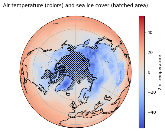
- sea_ice_cover
  (time, latitude, longitude)
  float32
  ...
  long_name :
  Sea ice area fraction
  short_name :
  siconc
  standard_name :
  sea_ice_area_fraction
  units :
  (0 - 1)
```
[769036826880 values with dtype=float32]
```
- sea_surface_temperature
  (time, latitude, longitude)
  float32
  ...
  long_name :
  Sea surface temperature
  short_name :
  sst
  units :
  K
```
[769036826880 values with dtype=float32]
```
- significant_height_of_combined_wind_waves_and_swell
  (time, latitude, longitude)
  float32
  ...
  long_name :
  Significant height of combined wind waves and swell
  short_name :
  swh
  units :
  m
```
[769036826880 values with dtype=float32]
```
- significant_height_of_total_swell
  (time, latitude, longitude)
  float32
  ...
  long_name :
  Significant height of total swell
  short_name :
  shts
  units :
  m
```
[769036826880 values with dtype=float32]
```
- significant_height_of_wind_waves
  (time, latitude, longitude)
  float32
  ...
  long_name :
  Significant height of wind waves
  short_name :
  shww
  units :
  m
```
[769036826880 values with dtype=float32]
```
- significant_wave_height_of_first_swell_partition
  (time, latitude, longitude)
  float32
  ...
  long_name :
  Significant wave height of first swell partition
  short_name :
  p140121
  units :
  m
```
[769036826880 values with dtype=float32]
```
- significant_wave_height_of_second_swell_partition
  (time, latitude, longitude)
  float32
  ...
  long_name :
  Significant wave height of second swell partition
  short_name :
  p140124
  units :
  m
```
[769036826880 values with dtype=float32]
```
- significant_wave_height_of_third_swell_partition
  (time, latitude, longitude)
  float32
  ...
  long_name :
  Significant wave height of third swell partition
  short_name :
  p140127
  units :
  m
```
[769036826880 values with dtype=float32]
```
- skin_reservoir_content
  (time, latitude, longitude)
  float32
  ...
  long_name :
  Skin reservoir content
  short_name :
  src
  units :
  m of water equivalent
```
[769036826880 values with dtype=float32]
```
- skin_temperature
  (time, latitude, longitude)
  float32
  ...
  long_name :
  Skin temperature
  short_name :
  skt
  units :
  K
```
[769036826880 values with dtype=float32]
```
- slope_of_sub_gridscale_orography
  (time, latitude, longitude)
  float32
  ...
  long_name :
  Slope of sub-gridscale orography
  short_name :
  slor
  units :
  ~
```
[769036826880 values with dtype=float32]
```
- snow_albedo
  (time, latitude, longitude)
  float32
  ...
  long_name :
  Snow albedo
  short_name :
  asn
  units :
  (0 - 1)
```
[769036826880 values with dtype=float32]
```
- snow_density
  (time, latitude, longitude)
  float32
  ...
  long_name :
  Snow density
  short_name :
  rsn
  units :
  kg m**-3
```
[769036826880 values with dtype=float32]
```
- snow_depth
  (time, latitude, longitude)
  float32
  ...
  long_name :
  Snow depth
  short_name :
  sd
  standard_name :
  lwe_thickness_of_surface_snow_amount
  units :
  m of water equivalent
```
[769036826880 values with dtype=float32]
```
- snow_evaporation
  (time, latitude, longitude)
  float32
  ...
  long_name :
  Snow evaporation
  short_name :
  es
  units :
  m of water equivalent
```
[769036826880 values with dtype=float32]
```
- snowfall
  (time, latitude, longitude)
  float32
  ...
  long_name :
  Snowfall
  short_name :
  sf
  standard_name :
  lwe_thickness_of_snowfall_amount
  units :
  m of water equivalent
```
[769036826880 values with dtype=float32]
```
- snowmelt
  (time, latitude, longitude)
  float32
  ...
  long_name :
  Snowmelt
  short_name :
  smlt
  units :
  m of water equivalent
```
[769036826880 values with dtype=float32]
```
- soil_temperature_level_1
  (time, latitude, longitude)
  float32
  ...
  long_name :
  Soil temperature level 1
  short_name :
  stl1
  standard_name :
  surface_temperature
  units :
  K
```
[769036826880 values with dtype=float32]
```
- soil_temperature_level_2
  (time, latitude, longitude)
  float32
  ...
  long_name :
  Soil temperature level 2
  short_name :
  stl2
  units :
  K
```
[769036826880 values with dtype=float32]
```
- soil_temperature_level_3
  (time, latitude, longitude)
  float32
  ...
  long_name :
  Soil temperature level 3
  short_name :
  stl3
  units :
  K
```
[769036826880 values with dtype=float32]
```
- soil_temperature_level_4
  (time, latitude, longitude)
  float32
  ...
  long_name :
  Soil temperature level 4
  short_name :
  stl4
  units :
  K
```
[769036826880 values with dtype=float32]
```
- soil_type
  (time, latitude, longitude)
  float32
  ...
  long_name :
  Soil type
  short_name :
  slt
  units :
  ~
```
[769036826880 values with dtype=float32]
```
- specific_cloud_ice_water_content
  (time, level, latitude, longitude)
  float32
  ...
  long_name :
  Specific cloud ice water content
  short_name :
  ciwc
  units :
  kg kg**-1
```
[28454362594560 values with dtype=float32]
```
- specific_cloud_liquid_water_content
  (time, level, latitude, longitude)
  float32
  ...
  long_name :
  Specific cloud liquid water content
  short_name :
  clwc
  units :
  kg kg**-1
```
[28454362594560 values with dtype=float32]
```
- specific_humidity
  (time, level, latitude, longitude)
  float32
  ...
  long_name :
  Specific humidity
  short_name :
  q
  standard_name :
  specific_humidity
  units :
  kg kg**-1
```
[28454362594560 values with dtype=float32]
```
- standard_deviation_of_filtered_subgrid_orography
  (time, latitude, longitude)
  float32
  ...
  long_name :
  Standard deviation of filtered subgrid orography
  short_name :
  sdfor
  units :
  m
```
[769036826880 values with dtype=float32]
```
- standard_deviation_of_orography
  (time, latitude, longitude)
  float32
  ...
  long_name :
  Standard deviation of orography
  short_name :
  sdor
  units :
  m
```
[769036826880 values with dtype=float32]
```
- sub_surface_runoff
  (time, latitude, longitude)
  float32
  ...
  long_name :
  Sub-surface runoff
  short_name :
  ssro
  units :
  m
```
[769036826880 values with dtype=float32]
```
- surface_latent_heat_flux
  (time, latitude, longitude)
  float32
  ...
  long_name :
  Surface latent heat flux
  short_name :
  slhf
  standard_name :
  surface_upward_latent_heat_flux
  units :
  J m**-2
```
[769036826880 values with dtype=float32]
```
- surface_net_solar_radiation
  (time, latitude, longitude)
  float32
  ...
  long_name :
  Surface net solar radiation
  short_name :
  ssr
  standard_name :
  surface_net_downward_shortwave_flux
  units :
  J m**-2
```
[769036826880 values with dtype=float32]
```
- surface_net_solar_radiation_clear_sky
  (time, latitude, longitude)
  float32
  ...
  long_name :
  Surface net solar radiation, clear sky
  short_name :
  ssrc
  standard_name :
  surface_net_downward_shortwave_flux_assuming_clear_sky
  units :
  J m**-2
```
[769036826880 values with dtype=float32]
```
- surface_net_thermal_radiation
  (time, latitude, longitude)
  float32
  ...
  long_name :
  Surface net thermal radiation
  short_name :
  str
  standard_name :
  surface_net_upward_longwave_flux
  units :
  J m**-2
```
[769036826880 values with dtype=float32]
```
- surface_net_thermal_radiation_clear_sky
  (time, latitude, longitude)
  float32
  ...
  long_name :
  Surface net thermal radiation, clear sky
  short_name :
  strc
  standard_name :
  surface_net_downward_longwave_flux_assuming_clear_sky
  units :
  J m**-2
```
[769036826880 values with dtype=float32]
```
- surface_pressure
  (time, latitude, longitude)
  float32
  ...
  long_name :
  Surface pressure
  short_name :
  sp
  standard_name :
  surface_air_pressure
  units :
  Pa
```
[769036826880 values with dtype=float32]
```
- surface_runoff
  (time, latitude, longitude)
  float32
  ...
  long_name :
  Surface runoff
  short_name :
  sro
  units :
  m
```
[769036826880 values with dtype=float32]
```
- surface_sensible_heat_flux
  (time, latitude, longitude)
  float32
  ...
  long_name :
  Surface sensible heat flux
  short_name :
  sshf
  standard_name :
  surface_upward_sensible_heat_flux
  units :
  J m**-2
```
[769036826880 values with dtype=float32]
```
- surface_solar_radiation_downward_clear_sky
  (time, latitude, longitude)
  float32
  ...
  long_name :
  Surface solar radiation downward clear-sky
  short_name :
  ssrdc
  units :
  J m**-2
```
[769036826880 values with dtype=float32]
```
- surface_solar_radiation_downwards
  (time, latitude, longitude)
  float32
  ...
  long_name :
  Surface solar radiation downwards
  short_name :
  ssrd
  standard_name :
  surface_downwelling_shortwave_flux_in_air
  units :
  J m**-2
```
[769036826880 values with dtype=float32]
```
- surface_thermal_radiation_downward_clear_sky
  (time, latitude, longitude)
  float32
  ...
  long_name :
  Surface thermal radiation downward clear-sky
  short_name :
  strdc
  units :
  J m**-2
```
[769036826880 values with dtype=float32]
```
- surface_thermal_radiation_downwards
  (time, latitude, longitude)
  float32
  ...
  long_name :
  Surface thermal radiation downwards
  short_name :
  strd
  units :
  J m**-2
```
[769036826880 values with dtype=float32]
```
- temperature
  (time, level, latitude, longitude)
  float32
  ...
  long_name :
  Temperature
  short_name :
  t
  standard_name :
  air_temperature
  units :
  K
```
[28454362594560 values with dtype=float32]
```
- temperature_of_snow_layer
  (time, latitude, longitude)
  float32
  ...
  long_name :
  Temperature of snow layer
  short_name :
  tsn
  standard_name :
  temperature_in_surface_snow
  units :
  K
```
[769036826880 values with dtype=float32]
```
- toa_incident_solar_radiation
  (time, latitude, longitude)
  float32
  ...
  long_name :
  TOA incident solar radiation
  short_name :
  tisr
  units :
  J m**-2
```
[769036826880 values with dtype=float32]
```
- top_net_solar_radiation
  (time, latitude, longitude)
  float32
  ...
  long_name :
  Top net solar radiation
  short_name :
  tsr
  standard_name :
  toa_net_upward_shortwave_flux
  units :
  J m**-2
```
[769036826880 values with dtype=float32]
```
- top_net_solar_radiation_clear_sky
  (time, latitude, longitude)
  float32
  ...
  long_name :
  Top net solar radiation, clear sky
  short_name :
  tsrc
  units :
  J m**-2
```
[769036826880 values with dtype=float32]
```
- top_net_thermal_radiation
  (time, latitude, longitude)
  float32
  ...
  long_name :
  Top net thermal radiation
  short_name :
  ttr
  standard_name :
  toa_outgoing_longwave_flux
  units :
  J m**-2
```
[769036826880 values with dtype=float32]
```
- top_net_thermal_radiation_clear_sky
  (time, latitude, longitude)
  float32
  ...
  long_name :
  Top net thermal radiation, clear sky
  short_name :
  ttrc
  units :
  J m**-2
```
[769036826880 values with dtype=float32]
```
- total_cloud_cover
  (time, latitude, longitude)
  float32
  ...
  long_name :
  Total cloud cover
  short_name :
  tcc
  standard_name :
  cloud_area_fraction
  units :
  (0 - 1)
```
[769036826880 values with dtype=float32]
```
- total_column_cloud_ice_water
  (time, latitude, longitude)
  float32
  ...
  long_name :
  Total column cloud ice water
  short_name :
  tciw
  units :
  kg m**-2
```
[769036826880 values with dtype=float32]
```
- total_column_cloud_liquid_water
  (time, latitude, longitude)
  float32
  ...
  long_name :
  Total column cloud liquid water
  short_name :
  tclw
  units :
  kg m**-2
```
[769036826880 values with dtype=float32]
```
- total_column_ozone
  (time, latitude, longitude)
  float32
  ...
  long_name :
  Total column ozone
  short_name :
  tco3
  standard_name :
  atmosphere_mass_content_of_ozone
  units :
  kg m**-2
```
[769036826880 values with dtype=float32]
```
- total_column_rain_water
  (time, latitude, longitude)
  float32
  ...
  long_name :
  Total column rain water
  short_name :
  tcrw
  units :
  kg m**-2
```
[769036826880 values with dtype=float32]
```
- total_column_snow_water
  (time, latitude, longitude)
  float32
  ...
  long_name :
  Total column snow water
  short_name :
  tcsw
  units :
  kg m**-2
```
[769036826880 values with dtype=float32]
```
- total_column_supercooled_liquid_water
  (time, latitude, longitude)
  float32
  ...
  long_name :
  Total column supercooled liquid water
  short_name :
  tcslw
  units :
  kg m**-2
```
[769036826880 values with dtype=float32]
```
- total_column_water
  (time, latitude, longitude)
  float32
  ...
  long_name :
  Total column water
  short_name :
  tcw
  units :
  kg m**-2
```
[769036826880 values with dtype=float32]
```
- total_column_water_vapour
  (time, latitude, longitude)
  float32
  ...
  long_name :
  Total column vertically-integrated water vapour
  short_name :
  tcwv
  standard_name :
  lwe_thickness_of_atmosphere_mass_content_of_water_vapor
  units :
  kg m**-2
```
[769036826880 values with dtype=float32]
```
- total_precipitation
  (time, latitude, longitude)
  float32
  ...
  long_name :
  Total precipitation
  short_name :
  tp
  units :
  m
```
[769036826880 values with dtype=float32]
```
- total_sky_direct_solar_radiation_at_surface
  (time, latitude, longitude)
  float32
  ...
  long_name :
  Total sky direct solar radiation at surface
  short_name :
  fdir
  units :
  J m**-2
```
[769036826880 values with dtype=float32]
```
- total_totals_index
  (time, latitude, longitude)
  float32
  ...
  long_name :
  Total totals index
  short_name :
  totalx
  units :
  K
```
[769036826880 values with dtype=float32]
```
- trapping_layer_base_height
  (time, latitude, longitude)
  float32
  ...
  long_name :
  Trapping layer base height
  short_name :
  tplb
  units :
  m
```
[769036826880 values with dtype=float32]
```
- trapping_layer_top_height
  (time, latitude, longitude)
  float32
  ...
  long_name :
  Trapping layer top height
  short_name :
  tplt
  units :
  m
```
[769036826880 values with dtype=float32]
```
- type_of_high_vegetation
  (time, latitude, longitude)
  float32
  ...
  long_name :
  Type of high vegetation
  short_name :
  tvh
  units :
  ~
```
[769036826880 values with dtype=float32]
```
- type_of_low_vegetation
  (time, latitude, longitude)
  float32
  ...
  long_name :
  Type of low vegetation
  short_name :
  tvl
  units :
  ~
```
[769036826880 values with dtype=float32]
```
- u_component_of_wind
  (time, level, latitude, longitude)
  float32
  ...
  long_name :
  U component of wind
  short_name :
  u
  standard_name :
  eastward_wind
  units :
  m s**-1
```
[28454362594560 values with dtype=float32]
```
- u_component_stokes_drift
  (time, latitude, longitude)
  float32
  ...
  long_name :
  U-component stokes drift
  short_name :
  ust
  units :
  m s**-1
```
[769036826880 values with dtype=float32]
```
- uv_visible_albedo_for_diffuse_radiation
  (time, latitude, longitude)
  float32
  ...
  long_name :
  UV visible albedo for diffuse radiation
  short_name :
  aluvd
  units :
  (0 - 1)
```
[769036826880 values with dtype=float32]
```
- uv_visible_albedo_for_direct_radiation
  (time, latitude, longitude)
  float32
  ...
  long_name :
  UV visible albedo for direct radiation
  short_name :
  aluvp
  units :
  (0 - 1)
```
[769036826880 values with dtype=float32]
```
- v_component_of_wind
  (time, level, latitude, longitude)
  float32
  ...
  long_name :
  V component of wind
  short_name :
  v
  standard_name :
  northward_wind
  units :
  m s**-1
```
[28454362594560 values with dtype=float32]
```
- v_component_stokes_drift
  (time, latitude, longitude)
  float32
  ...
  long_name :
  V-component stokes drift
  short_name :
  vst
  units :
  m s**-1
```
[769036826880 values with dtype=float32]
```
- vertical_integral_of_divergence_of_cloud_frozen_water_flux
  (time, latitude, longitude)
  float32
  ...
  long_name :
  Vertical integral of divergence of cloud frozen water flux
  short_name :
  p80.162
  units :
  kg m**-2 s**-1
```
[769036826880 values with dtype=float32]
```
- vertical_integral_of_divergence_of_cloud_liquid_water_flux
  (time, latitude, longitude)
  float32
  ...
  long_name :
  Vertical integral of divergence of cloud liquid water flux
  short_name :
  p79.162
  units :
  kg m**-2 s**-1
```
[769036826880 values with dtype=float32]
```
- vertical_integral_of_divergence_of_geopotential_flux
  (time, latitude, longitude)
  float32
  ...
  long_name :
  Vertical integral of divergence of geopotential flux
  short_name :
  p85.162
  units :
  W m**-2
```
[769036826880 values with dtype=float32]
```
- vertical_integral_of_divergence_of_kinetic_energy_flux
  (time, latitude, longitude)
  float32
  ...
  long_name :
  Vertical integral of divergence of kinetic energy flux
  short_name :
  p82.162
  units :
  W m**-2
```
[769036826880 values with dtype=float32]
```
- vertical_integral_of_divergence_of_mass_flux
  (time, latitude, longitude)
  float32
  ...
  long_name :
  Vertical integral of divergence of mass flux
  short_name :
  p81.162
  units :
  kg m**-2 s**-1
```
[769036826880 values with dtype=float32]
```
- vertical_integral_of_divergence_of_moisture_flux
  (time, latitude, longitude)
  float32
  ...
  long_name :
  Vertical integral of divergence of moisture flux
  short_name :
  p84.162
  units :
  kg m**-2 s**-1
```
[769036826880 values with dtype=float32]
```
- vertical_integral_of_divergence_of_ozone_flux
  (time, latitude, longitude)
  float32
  ...
  long_name :
  Vertical integral of divergence of ozone flux
  short_name :
  p87.162
  units :
  kg m**-2 s**-1
```
[769036826880 values with dtype=float32]
```
- vertical_integral_of_divergence_of_thermal_energy_flux
  (time, latitude, longitude)
  float32
  ...
  long_name :
  Vertical integral of divergence of thermal energy flux
  short_name :
  p83.162
  units :
  W m**-2
```
[769036826880 values with dtype=float32]
```
- vertical_integral_of_divergence_of_total_energy_flux
  (time, latitude, longitude)
  float32
  ...
  long_name :
  Vertical integral of divergence of total energy flux
  short_name :
  p86.162
  units :
  W m**-2
```
[769036826880 values with dtype=float32]
```
- vertical_integral_of_eastward_cloud_frozen_water_flux
  (time, latitude, longitude)
  float32
  ...
  long_name :
  Vertical integral of eastward cloud frozen water flux
  short_name :
  p90.162
  units :
  kg m**-1 s**-1
```
[769036826880 values with dtype=float32]
```
- vertical_integral_of_eastward_cloud_liquid_water_flux
  (time, latitude, longitude)
  float32
  ...
  long_name :
  Vertical integral of eastward cloud liquid water flux
  short_name :
  p88.162
  units :
  kg m**-1 s**-1
```
[769036826880 values with dtype=float32]
```
- vertical_integral_of_eastward_geopotential_flux
  (time, latitude, longitude)
  float32
  ...
  long_name :
  Vertical integral of eastward geopotential flux
  short_name :
  p73.162
  units :
  W m**-1
```
[769036826880 values with dtype=float32]
```
- vertical_integral_of_eastward_heat_flux
  (time, latitude, longitude)
  float32
  ...
  long_name :
  Vertical integral of eastward heat flux
  short_name :
  p69.162
  units :
  W m**-1
```
[769036826880 values with dtype=float32]
```
- vertical_integral_of_eastward_kinetic_energy_flux
  (time, latitude, longitude)
  float32
  ...
  long_name :
  Vertical integral of eastward kinetic energy flux
  short_name :
  p67.162
  units :
  W m**-1
```
[769036826880 values with dtype=float32]
```
- vertical_integral_of_eastward_mass_flux
  (time, latitude, longitude)
  float32
  ...
  long_name :
  Vertical integral of eastward mass flux
  short_name :
  p65.162
  units :
  kg m**-1 s**-1
```
[769036826880 values with dtype=float32]
```
- vertical_integral_of_eastward_ozone_flux
  (time, latitude, longitude)
  float32
  ...
  long_name :
  Vertical integral of eastward ozone flux
  short_name :
  p77.162
  units :
  kg m**-1 s**-1
```
[769036826880 values with dtype=float32]
```
- vertical_integral_of_eastward_total_energy_flux
  (time, latitude, longitude)
  float32
  ...
  long_name :
  Vertical integral of eastward total energy flux
  short_name :
  p75.162
  units :
  W m**-1
```
[769036826880 values with dtype=float32]
```
- vertical_integral_of_eastward_water_vapour_flux
  (time, latitude, longitude)
  float32
  ...
  long_name :
  Vertical integral of eastward water vapour flux
  short_name :
  p71.162
  units :
  kg m**-1 s**-1
```
[769036826880 values with dtype=float32]
```
- vertical_integral_of_energy_conversion
  (time, latitude, longitude)
  float32
  ...
  long_name :
  Vertical integral of energy conversion
  short_name :
  p64.162
  units :
  W m**-2
```
[769036826880 values with dtype=float32]
```
- vertical_integral_of_kinetic_energy
  (time, latitude, longitude)
  float32
  ...
  long_name :
  Vertical integral of kinetic energy
  short_name :
  p59.162
  units :
  J m**-2
```
[769036826880 values with dtype=float32]
```
- vertical_integral_of_mass_of_atmosphere
  (time, latitude, longitude)
  float32
  ...
  long_name :
  Vertical integral of mass of atmosphere
  short_name :
  p53.162
  units :
  kg m**-2
```
[769036826880 values with dtype=float32]
```
- vertical_integral_of_mass_tendency
  (time, latitude, longitude)
  float32
  ...
  long_name :
  Vertical integral of mass tendency
  short_name :
  p92.162
  units :
  kg m**-2 s**-1
```
[769036826880 values with dtype=float32]
```
- vertical_integral_of_northward_cloud_frozen_water_flux
  (time, latitude, longitude)
  float32
  ...
  long_name :
  Vertical integral of northward cloud frozen water flux
  short_name :
  p91.162
  units :
  kg m**-1 s**-1
```
[769036826880 values with dtype=float32]
```
- vertical_integral_of_northward_cloud_liquid_water_flux
  (time, latitude, longitude)
  float32
  ...
  long_name :
  Vertical integral of northward cloud liquid water flux
  short_name :
  p89.162
  units :
  kg m**-1 s**-1
```
[769036826880 values with dtype=float32]
```
- vertical_integral_of_northward_geopotential_flux
  (time, latitude, longitude)
  float32
  ...
  long_name :
  Vertical integral of northward geopotential flux
  short_name :
  p74.162
  units :
  W m**-1
```
[769036826880 values with dtype=float32]
```
- vertical_integral_of_northward_heat_flux
  (time, latitude, longitude)
  float32
  ...
  long_name :
  Vertical integral of northward heat flux
  short_name :
  p70.162
  units :
  W m**-1
```
[769036826880 values with dtype=float32]
```
- vertical_integral_of_northward_kinetic_energy_flux
  (time, latitude, longitude)
  float32
  ...
  long_name :
  Vertical integral of northward kinetic energy flux
  short_name :
  p68.162
  units :
  W m**-1
```
[769036826880 values with dtype=float32]
```
- vertical_integral_of_northward_mass_flux
  (time, latitude, longitude)
  float32
  ...
  long_name :
  Vertical integral of northward mass flux
  short_name :
  p66.162
  units :
  kg m**-1 s**-1
```
[769036826880 values with dtype=float32]
```
- vertical_integral_of_northward_ozone_flux
  (time, latitude, longitude)
  float32
  ...
  long_name :
  Vertical integral of northward ozone flux
  short_name :
  p78.162
  units :
  kg m**-1 s**-1
```
[769036826880 values with dtype=float32]
```
- vertical_integral_of_northward_total_energy_flux
  (time, latitude, longitude)
  float32
  ...
  long_name :
  Vertical integral of northward total energy flux
  short_name :
  p76.162
  units :
  W m**-1
```
[769036826880 values with dtype=float32]
```
- vertical_integral_of_northward_water_vapour_flux
  (time, latitude, longitude)
  float32
  ...
  long_name :
  Vertical integral of northward water vapour flux
  short_name :
  p72.162
  units :
  kg m**-1 s**-1
```
[769036826880 values with dtype=float32]
```
- vertical_integral_of_potential_and_internal_energy
  (time, latitude, longitude)
  float32
  ...
  long_name :
  Vertical integral of potential+internal energy
  short_name :
  p61.162
  units :
  J m**-2
```
[769036826880 values with dtype=float32]
```
- vertical_integral_of_potential_internal_and_latent_energy
  (time, latitude, longitude)
  float32
  ...
  long_name :
  Vertical integral of potential+internal+latent energy
  short_name :
  p62.162
  units :
  J m**-2
```
[769036826880 values with dtype=float32]
```
- vertical_integral_of_temperature
  (time, latitude, longitude)
  float32
  ...
  long_name :
  Vertical integral of temperature
  short_name :
  p54.162
  units :
  K kg m**-2
```
[769036826880 values with dtype=float32]
```
- vertical_integral_of_thermal_energy
  (time, latitude, longitude)
  float32
  ...
  long_name :
  Vertical integral of thermal energy
  short_name :
  p60.162
  units :
  J m**-2
```
[769036826880 values with dtype=float32]
```
- vertical_integral_of_total_energy
  (time, latitude, longitude)
  float32
  ...
  long_name :
  Vertical integral of total energy
  short_name :
  p63.162
  units :
  J m**-2
```
[769036826880 values with dtype=float32]
```
- vertical_velocity
  (time, level, latitude, longitude)
  float32
  ...
  long_name :
  Vertical velocity
  short_name :
  w
  standard_name :
  lagrangian_tendency_of_air_pressure
  units :
  Pa s**-1
```
[28454362594560 values with dtype=float32]
```
- vertically_integrated_moisture_divergence
  (time, latitude, longitude)
  float32
  ...
  long_name :
  Vertically integrated moisture divergence
  short_name :
  vimd
  units :
  kg m**-2
```
[769036826880 values with dtype=float32]
```
- volumetric_soil_water_layer_1
  (time, latitude, longitude)
  float32
  ...
  long_name :
  Volumetric soil water layer 1
  short_name :
  swvl1
  units :
  m**3 m**-3
```
[769036826880 values with dtype=float32]
```
- volumetric_soil_water_layer_2
  (time, latitude, longitude)
  float32
  ...
  long_name :
  Volumetric soil water layer 2
  short_name :
  swvl2
  units :
  m**3 m**-3
```
[769036826880 values with dtype=float32]
```
- volumetric_soil_water_layer_3
  (time, latitude, longitude)
  float32
  ...
  long_name :
  Volumetric soil water layer 3
  short_name :
  swvl3
  units :
  m**3 m**-3
```
[769036826880 values with dtype=float32]
```
- volumetric_soil_water_layer_4
  (time, latitude, longitude)
  float32
  ...
  long_name :
  Volumetric soil water layer 4
  short_name :
  swvl4
  units :
  m**3 m**-3
```
[769036826880 values with dtype=float32]
```
- wave_spectral_directional_width
  (time, latitude, longitude)
  float32
  ...
  long_name :
  Wave spectral directional width
  short_name :
  wdw
  units :
  radians
```
[769036826880 values with dtype=float32]
```
- wave_spectral_directional_width_for_swell
  (time, latitude, longitude)
  float32
  ...
  long_name :
  Wave spectral directional width for swell
  short_name :
  dwps
  units :
  radians
```
[769036826880 values with dtype=float32]
```
- wave_spectral_directional_width_for_wind_waves
  (time, latitude, longitude)
  float32
  ...
  long_name :
  Wave spectral directional width for wind waves
  short_name :
  dwww
  units :
  radians
```
[769036826880 values with dtype=float32]
```
- wave_spectral_kurtosis
  (time, latitude, longitude)
  float32
  ...
  long_name :
  Wave spectral kurtosis
  short_name :
  wsk
  units :
  dimensionless
```
[769036826880 values with dtype=float32]
```
- wave_spectral_peakedness
  (time, latitude, longitude)
  float32
  ...
  long_name :
  Wave spectral peakedness
  short_name :
  wsp
  units :
  dimensionless
```
[769036826880 values with dtype=float32]
```
- wave_spectral_skewness
  (time, latitude, longitude)
  float32
  ...
  long_name :
  Wave Spectral Skewness
  short_name :
  wss
  units :
  dimensionless
```
[769036826880 values with dtype=float32]
```
- zero_degree_level
  (time, latitude, longitude)
  float32
  ...
  long_name :
  0 degrees C isothermal level (atm)
  short_name :
  deg0l
  units :
  m
```
[769036826880 values with dtype=float32]
```

Indexes: (4)

latitude

PandasIndex

PandasIndex(Index([  90.0,  89.75,   89.5,  89.25,   89.0,  88.75,   88.5,  88.25,   88.0,
        87.75,
       ...
       -87.75,  -88.0, -88.25,  -88.5, -88.75,  -89.0, -89.25,  -89.5, -89.75,
        -90.0],
      dtype='float32', name='latitude', length=721))

level

PandasIndex

PandasIndex(Index([   1,    2,    3,    5,    7,   10,   20,   30,   50,   70,  100,  125,
        150,  175,  200,  225,  250,  300,  350,  400,  450,  500,  550,  600,
        650,  700,  750,  775,  800,  825,  850,  875,  900,  925,  950,  975,
       1000],
      dtype='int64', name='level'))

longitude

PandasIndex

PandasIndex(Index([   0.0,   0.25,    0.5,   0.75,    1.0,   1.25,    1.5,   1.75,    2.0,
         2.25,
       ...
        357.5, 357.75,  358.0, 358.25,  358.5, 358.75,  359.0, 359.25,  359.5,
       359.75],
      dtype='float32', name='longitude', length=1440))

time

PandasIndex

PandasIndex(DatetimeIndex(['1940-01-01 00:00:00', '1940-01-01 01:00:00',
               '1940-01-01 02:00:00', '1940-01-01 03:00:00',
               '1940-01-01 04:00:00', '1940-01-01 05:00:00',
               '1940-01-01 06:00:00', '1940-01-01 07:00:00',
               '1940-01-01 08:00:00', '1940-01-01 09:00:00',
               ...
               '2024-06-30 14:00:00', '2024-06-30 15:00:00',
               '2024-06-30 16:00:00', '2024-06-30 17:00:00',
               '2024-06-30 18:00:00', '2024-06-30 19:00:00',
               '2024-06-30 20:00:00', '2024-06-30 21:00:00',
               '2024-06-30 22:00:00', '2024-06-30 23:00:00'],
              dtype='datetime64[ns]', name='time', length=740712, freq=None))

Attributes: (3)
valid_time_start :
1940-01-01
last_updated :
2024-09-27 08:06:09.120900
valid_time_stop :
2024-06-30

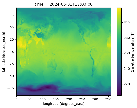
With xarray we can quite quickly make a selection of the data (here a certain point in time), and plot it.

Note that only once the actual underlying data is needed for creating output, such as plotting, the data is retrieved from Google’s servers:

ar_full_37_1h["2m_temperature"].sel(time="2024-05-01T12:00:00").plot()

<matplotlib.collections.QuadMesh at 0x132367410>

_images/a6495d3e77eba3926271d178a6cdbe1739987433601016d1021e2dc90dd5fa2c.png

Caveats with using the ARCO-ERA5 dataset#

One main drawback of the ARCO-ERA5 dataset is how the data is organized. Data is stored in blocks called “chunks”, which is a manageable piece of a larger dataset. They are often used to store information about specific topics or categories.

When retrieving data, the whole chunk has to be retrieved. Partial retrieval of chunks is not possible.

The ARCO-ERA5 dataset is organized like the following illustration:

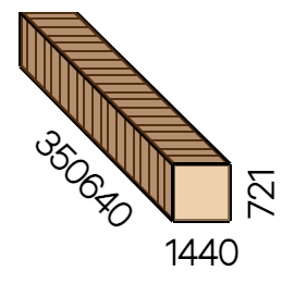
Where the latitude and longitude dimensions (sizes 721 and 1440 respectively) are all in the same chunk, while each time step is on a separate chunk. When you want to retrieve data for a single lat/lon, for example, a timeseries of air temperature near Leiden, the Netherlands, every single chunk of the entire air temperature array has to be downloaded.

There are tools such as Rechunker which can reorganize the data for you, but this requires storing a copy of the data elsewhere.

Demonstration of chunk issue#

The code cell below demonstrates the problem. We request the air temperature data for the data point closest to leiden, but only one out of every 720 timesteps (approximately a month), for the years 2000-2020

This still means we need to download 12 timesteps per year, for 20 years, i.e., 240 chunks. Which is hundreds of megabytes just for a simple timeseries.

loc_leiden = {"latitude": 52.17, "longitude": 4.46}

# Select every 30th day of data to reduce the number of chunks that need to be downloaded
monthly_temperature = ar_full_37_1h["2m_temperature"].isel(time=slice(None, None, 24*30))
monthly_temperature = monthly_temperature.sel(time=slice("2000-01-01", "2020-01-01"))
monthly_temperature.sel(loc_leiden, method="nearest").plot()

[<matplotlib.lines.Line2D at 0x10e3574d0>]

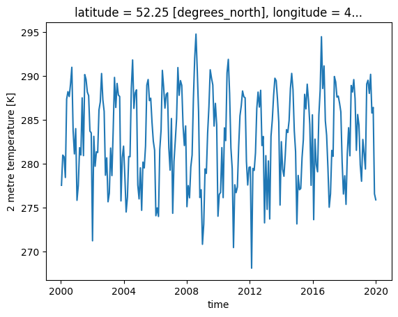
_images/d4157f59746db388e0756ba41518cc09305e9dd979469b3f44c93f23ad57d90f.png

Prettier plots#

The main showcase of the Zarr ARCO-ERA5 dataset has ended. However, below are included some examples to show off the plotting and analysis possiblities.

Air temperature on an orthographic projection#

We can make this plot a bit prettier by making use of cartopy:

# First we may need to install cartopy
%pip install cartopy

import cartopy.crs as ccrs
import matplotlib.pyplot as plt

ax = plt.axes(projection=ccrs.Orthographic(0, 25))
ax.gridlines()
ax.coastlines()

ds_t = ar_full_37_1h["2m_temperature"].sel(time="2024-01-01T00:00:00")

(ds_t - 273.15).plot(
    ax=ax, cmap="coolwarm", transform=ccrs.PlateCarree()
)

<cartopy.mpl.geocollection.GeoQuadMesh at 0x110758c10>

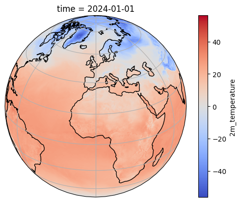
_images/c8f66925e724e8f204aec20cde7f94352e0d0f92313d696efc08289b039b9b60.png

Air temperature and sea-ice cover#

We can also add additional information to the plot such as sea-ice cover:

ax = plt.axes(projection=ccrs.Orthographic(0, 90))
ax.gridlines()
ax.coastlines()

ds_ice = ar_full_37_1h["sea_ice_cover"].sel(time="2024-01-01T00:00:00")

(ds_t - 273.15).plot(
    ax=ax, cmap="coolwarm", transform=ccrs.PlateCarree()
)
ds_ice.where(ds_ice>0.2).plot.contourf(
    colors=[(1, 1, 1, 0.0)],  # RGBA color (alpha is 0.0 to make it transparent)
    ax=ax, transform=ccrs.PlateCarree(), hatches=['xxxxx'], add_colorbar=False,
)
plt.title("Air temperature (colors) and sea ice cover (hatched area)\n")

Text(0.5, 1.0, 'Air temperature (colors) and sea ice cover (hatched area)\n')

_images/c45d9e9e1d5fd54315e3fbf17516b18034ebd81cad2d2b2a8fe8f886e795f658.png

Cloud Optimized ERA5

Contents

Cloud Optimized ERA5#

Accessing the dataset#

How to use xarray with Zarr stores#

Caveats with using the ARCO-ERA5 dataset#

Demonstration of chunk issue#

Prettier plots#

Air temperature on an orthographic projection#

Air temperature and sea-ice cover#