Dask: lazy and distributed compute#
For this notebook to run, we can make sure all required packages are installed
%pip install dask[distributed] xarray xarray_regrid matplotlib
Lazy computation#
Using xarray and Dask it is possible to perform computations “lazily”. Lazy computation is when you only load data and perform the computations once it is required.
For example, let’s define two functions, and apply these to x:
def inc(i):
    return i + 1

def add(a, b):
    return a + b

x = 1
y = inc(x)
z = add(y, 10)
From these operations, Dask will create a so-called ‘task graph’ that stores which operations need to be performed on x:
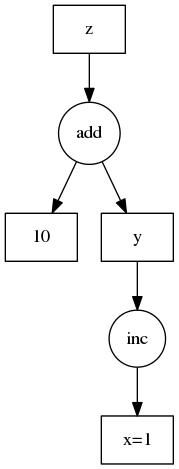
Dask will execute the graph and return the result, only once you specifically ask for it:
z.compute()
Example code and image originate from the Dask documentation, Copyright (c) 2014, Anaconda, Inc. and contributors
We can actually run this example if we tell Dask to delay the execution.
import dask

@dask.delayed
def inc(i):
    return i + 1

@dask.delayed
def add(a, b):
    return a + b

x = 1
y = inc(x)
z = add(y, 10)
z  # returns 'delayed' object
Delayed('add-5a0ec4f9-a156-40bc-8bdf-5da5e0fbcb24')
We can compute the result by calling .compute():
z.compute()
12
Distributed computing#
Dask also allows distributed computing of tasks. Tasks will be distributed over multiple cores, and the results aggregated. This allows you to relatively easily speed up computations.
The computations can be spread over local cores, but can also be performed on cloud infrastructure instead.
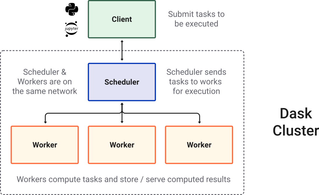
Image originates from the Dask documentation, Copyright (c) 2014, Anaconda, Inc. and contributors
import dask.distributed

client = dask.distributed.Client() # You can also connect to a remote/cloud server here instead
client  # Show the client
Client
Client-b28cb7d9-8a1c-11ef-97b3-d1d1712b09fe
| Connection method: Cluster object | Cluster type: distributed.LocalCluster |
| Dashboard: http://127.0.0.1:8787/status |
Cluster Info
LocalCluster
22ee443d
| Dashboard: http://127.0.0.1:8787/status | Workers: 4 |
| Total threads: 8 | Total memory: 15.33 GiB |
| Status: running | Using processes: True |
Scheduler Info
Scheduler
Scheduler-d6aca045-4c16-40c0-9f50-7e0c2187d9c2
| Comm: tcp://127.0.0.1:44509 | Workers: 4 |
| Dashboard: http://127.0.0.1:8787/status | Total threads: 8 |
| Started: Just now | Total memory: 15.33 GiB |
Workers
Worker: 0
| Comm: tcp://127.0.0.1:46459 | Total threads: 2 |
| Dashboard: http://127.0.0.1:42103/status | Memory: 3.83 GiB |
| Nanny: tcp://127.0.0.1:42929 | |
| Local directory: /tmp/dask-scratch-space/worker-d0q323nm | |
Worker: 1
| Comm: tcp://127.0.0.1:35857 | Total threads: 2 |
| Dashboard: http://127.0.0.1:33089/status | Memory: 3.83 GiB |
| Nanny: tcp://127.0.0.1:39891 | |
| Local directory: /tmp/dask-scratch-space/worker-blyecc1r | |
Worker: 2
| Comm: tcp://127.0.0.1:42767 | Total threads: 2 |
| Dashboard: http://127.0.0.1:35845/status | Memory: 3.83 GiB |
| Nanny: tcp://127.0.0.1:36507 | |
| Local directory: /tmp/dask-scratch-space/worker-xrm95ijj | |
Worker: 3
| Comm: tcp://127.0.0.1:36795 | Total threads: 2 |
| Dashboard: http://127.0.0.1:38189/status | Memory: 3.83 GiB |
| Nanny: tcp://127.0.0.1:46601 | |
| Local directory: /tmp/dask-scratch-space/worker-34ogk9ta | |
Regridding example#
Projecting data on different grids is a common operation in geosciences. The original data might be of a too high resolution to work with, or you are collecting data from multiple sources and need a common grid to compare or aggregate them.
In the EXCITED project we developed a tool for this to perform regridding in xarray, which can make full use of Dask.
Sea surface temperature dataset#
In this example we’ll use a sea surface temperature (SST) dataset, which is available at a very high resolution:
import xarray as xr
sst = xr.open_zarr("https://mur-sst.s3.us-west-2.amazonaws.com/zarr-v1")["analysed_sst"]
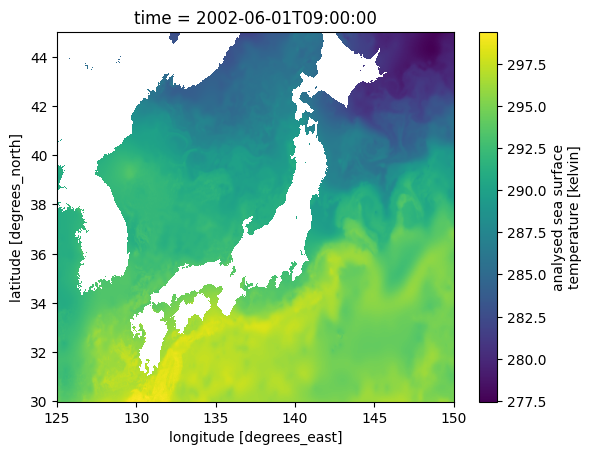
# Reduce size of array by only selecting a slice
sst.sel(lat=slice(30, 45), lon=slice(125, 150)).isel(time=0).plot()
<matplotlib.collections.QuadMesh at 0x14f575390>
Note that the full DataArray contains 30 terabytes (!) of data:
sst
<xarray.DataArray 'analysed_sst' (time: 6443, lat: 17999, lon: 36000)> Size: 33TB
dask.array<open_dataset-analysed_sst, shape=(6443, 17999, 36000), dtype=float64, chunksize=(5, 1799, 3600), chunktype=numpy.ndarray>
Coordinates:
  * lat      (lat) float32 72kB -89.99 -89.98 -89.97 ... 89.97 89.98 89.99
  * lon      (lon) float32 144kB -180.0 -180.0 -180.0 ... 180.0 180.0 180.0
  * time     (time) datetime64[ns] 52kB 2002-06-01T09:00:00 ... 2020-01-20T09...
Attributes:
    comment:        "Final" version using Multi-Resolution Variational Analys...
    long_name:      analysed sea surface temperature
    standard_name:  sea_surface_foundation_temperature
    units:          kelvin
    valid_max:      32767
valid_min: -32767Regridding lazily#
We can define a new grid, this time at a lower resolution to match other datasets (e.g. ERA5). We can also define the spatial bounds of this new grid:
import xarray_regrid

target = xarray_regrid.Grid(
    north=45,
    south=30,
    west=125,
    east=150,
    resolution_lat=0.25,
    resolution_lon=0.25,
).create_regridding_dataset(lat_name="lat", lon_name="lon")
With this target grid we can regrid the data. Running it will only take a few seconds, however, no computations are performed yet.
Dask will store the regridding operation, and regridding will only be applied to the (required) data afterwards:
# use a binning strategy, taking the mean of the bins
sst_regrid = sst.regrid.stat(target, method="mean")
sst_regrid # note that the new object has a much lower resolution, but is not computed yet
<xarray.DataArray 'analysed_sst' (time: 6443, lat: 61, lon: 101)> Size: 318MB
dask.array<transpose, shape=(6443, 61, 101), dtype=float64, chunksize=(5, 61, 101), chunktype=numpy.ndarray>
Coordinates:
  * time     (time) datetime64[ns] 52kB 2002-06-01T09:00:00 ... 2020-01-20T09...
  * lon      (lon) float64 808B 125.0 125.2 125.5 125.8 ... 149.5 149.8 150.0
  * lat      (lat) float64 488B 30.0 30.25 30.5 30.75 ... 44.25 44.5 44.75 45.0
Attributes:
    comment:        "Final" version using Multi-Resolution Variational Analys...
    long_name:      analysed sea surface temperature
    standard_name:  sea_surface_foundation_temperature
    units:          kelvin
    valid_max:      32767
valid_min: -32767Only once the following cell is run, will the regridding operation be performed on this slice of data.
Dask will automatically spread the computation over multiple cores.
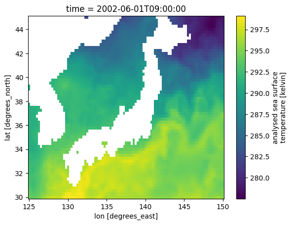
sst_regrid.isel(time=0).plot()
/Users/clairedonnelly/workshop_tutorial/.venv/lib/python3.11/site-packages/distributed/client.py:3361: UserWarning: Sending large graph of size 30.26 MiB.
This may cause some slowdown.
Consider loading the data with Dask directly
 or using futures or delayed objects to embed the data into the graph without repetition.
See also https://docs.dask.org/en/stable/best-practices.html#load-data-with-dask for more information.
  warnings.warn(
<matplotlib.collections.QuadMesh at 0x2f19c9690>