Zarr store for FLUXNET2015

The FLUXNET2015 dataset is an amazing collection of site data from multiple regional flux networks. The data collection and analysis represents the efforts of hundreds of scientists and technicians around the world, and has broad applications ranging from ecophysiology studies, remote sensing studies, and development of ecosystem and Earth system models.

Usually, to get the data, you would:

1. go to the FLUXNET organization website

2. create an account

3. select the data product, and mark the sites you are interested in

4. agree to the data policy and request the download

5. wait for the download to be prepared

6. click on the download links for every individual site

7. extract the .zip files

8. read in the CSV files

This is not a very streamlined process. Additionally, due to the nature of CSV files, the metadata is included in a separate file and not with the data.

As a demo, we converted part of the “tier one” (CC-BY-4.0 licensed) FLUXNET2015 dataset to a Zarr store, which is a community-driven data format for chunked, compressed, N-dimensional arrays (such as numpy arrays) based on an open-source specification. Using a Zarr store makes it easier for users to access data and reproduce research.

Accessing the dataset

Before opening the dataset, you might need to install the following dependencies:

%pip install xarray zarr aiohttp requests 
%pip install "dask[diagnostics]" --upgrade

To open the data using xarray in Python, we need to specify the link to the zarr store and how the data should be chunked. In this case, we are chunking the data by site:

import xarray as xr

ds = xr.open_dataset(
    "https://excited-co2.github.io/zarr-fluxnet2015/fluxnet.zarr",
    chunks={"time": -1, "site": 1},  # Data is chunked by site
)

Selecting and displaying data

Once opened, we can view the whole dataset. It includes six variables and their quality flags. By clicking on the icon, you can view the attributes of a variable.

The dataset level attributes (title, citation, etc.) are listed at the bottom.

ds

<xarray.Dataset> Size: 7GB
Dimensions:    (site: 204, time: 420775)
Coordinates:
  * site       (site) <U6 5kB 'US-Myb' 'CA-SF1' 'US-Twt' ... 'SJ-Blv' 'FR-Pue'
  * time       (time) datetime64[ns] 3MB 1991-01-01T06:00:00 ... 2015-01-01T0...
Data variables:
    gpp_dt     (site, time) float64 687MB dask.array<chunksize=(1, 420775), meta=np.ndarray>
    gpp_nt     (site, time) float64 687MB dask.array<chunksize=(1, 420775), meta=np.ndarray>
    latitude   (site) float64 2kB dask.array<chunksize=(1,), meta=np.ndarray>
    longitude  (site) float64 2kB dask.array<chunksize=(1,), meta=np.ndarray>
    nee        (site, time) float64 687MB dask.array<chunksize=(1, 420775), meta=np.ndarray>
    nee_qc     (site, time) float64 687MB dask.array<chunksize=(1, 420775), meta=np.ndarray>
    sw_in      (site, time) float64 687MB dask.array<chunksize=(1, 420775), meta=np.ndarray>
    sw_in_qc   (site, time) float64 687MB dask.array<chunksize=(1, 420775), meta=np.ndarray>
    ta         (site, time) float64 687MB dask.array<chunksize=(1, 420775), meta=np.ndarray>
    ta_qc      (site, time) float64 687MB dask.array<chunksize=(1, 420775), meta=np.ndarray>
    vpd        (site, time) float64 687MB dask.array<chunksize=(1, 420775), meta=np.ndarray>
    vpd_qc     (site, time) float64 687MB dask.array<chunksize=(1, 420775), meta=np.ndarray>
Attributes:
    Conventions:             None
    attribution_guidelines:  - Cite the data-collection paper, i.e., cite Pas...
    citation:                Pastorello, G., Trotta, C., Canfora, E. et al. T...
    description:             The FLUXNET2015 Dataset includes data collected ...
    doi:                     https://doi.org/10.1038/s41597-020-0534-3
    history:                 Converted from FULLSET FLUXNET2015 to Zarr on 20...
    license:                 CC-BY-4.0
    title:                   FLUXNET2015 Dataset

xarray.Dataset

• Dimensions:
  • site: 204
  • time: 420775
• Coordinates: (2)
  • site
    (site)
    <U6
    'US-Myb' 'CA-SF1' ... 'FR-Pue'

    long_name :

    Fluxnet site code

    array(['US-Myb', 'CA-SF1', 'US-Twt', ..., 'IT-Cp2', 'SJ-Blv', 'FR-Pue'],
          dtype='<U6')

  • time
    (time)
    datetime64[ns]
    1991-01-01T06:00:00 ... 2015-01-...

    array(['1991-01-01T06:00:00.000000000', '1991-01-01T06:30:00.000000000',
           '1991-01-01T07:00:00.000000000', ..., '2015-01-01T08:00:00.000000000',
           '2015-01-01T08:30:00.000000000', '2015-01-01T09:00:00.000000000'],
          dtype='datetime64[ns]')

• Data variables: (12)
  • gpp_dt
    (site, time)
    float64
    dask.array<chunksize=(1, 420775), meta=np.ndarray>

    long_name :

    gross primary production (daytime partitioning method)

    units :

    umolCO2 m-2 s-1

    Array Chunk Bytes 654.89 MiB 3.21 MiB Shape (204, 420775) (1, 420775) Dask graph 204 chunks in 2 graph layers Data type float64 numpy.ndarray

  • gpp_nt
    (site, time)
    float64
    dask.array<chunksize=(1, 420775), meta=np.ndarray>

    long_name :

    gross primary production (nighttime partitioning method)

    units :

    umolCO2 m-2 s-1

    Array Chunk Bytes 654.89 MiB 3.21 MiB Shape (204, 420775) (1, 420775) Dask graph 204 chunks in 2 graph layers Data type float64 numpy.ndarray

  • latitude
    (site)
    float64
    dask.array<chunksize=(1,), meta=np.ndarray>

    long_name :

    Fluxnet site latitude

    units :

    degrees_north

    Array Chunk Bytes 1.59 kiB 8 B Shape (204,) (1,) Dask graph 204 chunks in 2 graph layers Data type float64 numpy.ndarray

  • longitude
    (site)
    float64
    dask.array<chunksize=(1,), meta=np.ndarray>

    long_name :

    Fluxnet site longitude

    units :

    degrees_east

    Array Chunk Bytes 1.59 kiB 8 B Shape (204,) (1,) Dask graph 204 chunks in 2 graph layers Data type float64 numpy.ndarray

  • nee
    (site, time)
    float64
    dask.array<chunksize=(1, 420775), meta=np.ndarray>

    long_name :

    net ecosystem exchange

    units :

    umolCO2 m-2 s-1

    Array Chunk Bytes 654.89 MiB 3.21 MiB Shape (204, 420775) (1, 420775) Dask graph 204 chunks in 2 graph layers Data type float64 numpy.ndarray

  • nee_qc
    (site, time)
    float64
    dask.array<chunksize=(1, 420775), meta=np.ndarray>

    long_name :

    net ecosystem exchange quality flag

    Array Chunk Bytes 654.89 MiB 3.21 MiB Shape (204, 420775) (1, 420775) Dask graph 204 chunks in 2 graph layers Data type float64 numpy.ndarray

  • sw_in
    (site, time)
    float64
    dask.array<chunksize=(1, 420775), meta=np.ndarray>

    long_name :

    incoming shortwave radiation

    units :

    W m-2

    Array Chunk Bytes 654.89 MiB 3.21 MiB Shape (204, 420775) (1, 420775) Dask graph 204 chunks in 2 graph layers Data type float64 numpy.ndarray

  • sw_in_qc
    (site, time)
    float64
    dask.array<chunksize=(1, 420775), meta=np.ndarray>

    long_name :

    incoming shortwave radiation quality flag

    Array Chunk Bytes 654.89 MiB 3.21 MiB Shape (204, 420775) (1, 420775) Dask graph 204 chunks in 2 graph layers Data type float64 numpy.ndarray

  • ta
    (site, time)
    float64
    dask.array<chunksize=(1, 420775), meta=np.ndarray>

    long_name :

    air temperature

    units :

    degC

    Array Chunk Bytes 654.89 MiB 3.21 MiB Shape (204, 420775) (1, 420775) Dask graph 204 chunks in 2 graph layers Data type float64 numpy.ndarray

  • ta_qc
    (site, time)
    float64
    dask.array<chunksize=(1, 420775), meta=np.ndarray>

    long_name :

    air temperature quality flag

    Array Chunk Bytes 654.89 MiB 3.21 MiB Shape (204, 420775) (1, 420775) Dask graph 204 chunks in 2 graph layers Data type float64 numpy.ndarray

  • vpd
    (site, time)
    float64
    dask.array<chunksize=(1, 420775), meta=np.ndarray>

    long_name :

    vapor pressure deficit

    units :

    kPa

    Array Chunk Bytes 654.89 MiB 3.21 MiB Shape (204, 420775) (1, 420775) Dask graph 204 chunks in 2 graph layers Data type float64 numpy.ndarray

  • vpd_qc
    (site, time)
    float64
    dask.array<chunksize=(1, 420775), meta=np.ndarray>

    long_name :

    vapor pressure deficit quality flag

    Array Chunk Bytes 654.89 MiB 3.21 MiB Shape (204, 420775) (1, 420775) Dask graph 204 chunks in 2 graph layers Data type float64 numpy.ndarray

• Indexes: (2)
  • site
    PandasIndex

    PandasIndex(Index(['US-Myb', 'CA-SF1', 'US-Twt', 'US-ARc', 'GL-NuF', 'DE-Obe', 'DE-Tha',
           'US-Sta', 'US-Wi8', 'AU-DaP',
           ...
           'FR-Gri', 'CN-Din', 'CH-Lae', 'CH-Cha', 'CA-TP3', 'FI-Hyy', 'CA-SF2',
           'IT-Cp2', 'SJ-Blv', 'FR-Pue'],
          dtype='object', name='site', length=204))

  • time
    PandasIndex

    PandasIndex(DatetimeIndex(['1991-01-01 06:00:00', '1991-01-01 06:30:00',
                   '1991-01-01 07:00:00', '1991-01-01 07:30:00',
                   '1991-01-01 08:00:00', '1991-01-01 08:30:00',
                   '1991-01-01 09:00:00', '1991-01-01 09:30:00',
                   '1991-01-01 10:00:00', '1991-01-01 10:30:00',
                   ...
                   '2015-01-01 04:30:00', '2015-01-01 05:00:00',
                   '2015-01-01 05:30:00', '2015-01-01 06:00:00',
                   '2015-01-01 06:30:00', '2015-01-01 07:00:00',
                   '2015-01-01 07:30:00', '2015-01-01 08:00:00',
                   '2015-01-01 08:30:00', '2015-01-01 09:00:00'],
                  dtype='datetime64[ns]', name='time', length=420775, freq=None))

• Attributes: (8)

  Conventions :

  None

  attribution_guidelines :

  - Cite the data-collection paper, i.e., cite Pastorello et al. 20201. - List each site used by its FLUXNET ID and/or per-site DOIs in the paper.

  citation :

  Pastorello, G., Trotta, C., Canfora, E. et al. The FLUXNET2015 dataset and the ONEFlux processing pipeline for eddy covariance data. Sci Data 7, 225 (2020).

  description :

  The FLUXNET2015 Dataset includes data collected at sites from multiple regional flux networks. The preparation of this FLUXNET Dataset has been possible thanks only to the efforts of many scientists and technicians around the world and the coordination among teams from regional networks.

  doi :

  https://doi.org/10.1038/s41597-020-0534-3

  history :

  Converted from FULLSET FLUXNET2015 to Zarr on 2024-10-08 14:39:35.139665+00:00.

  license :

  CC-BY-4.0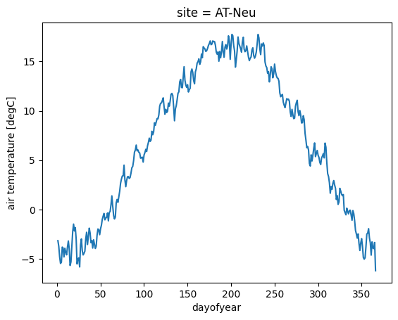

  title :

  FLUXNET2015 Dataset

We can now access the variables and plot the data using xarray. As an example, here we plot the mean for each day for the “air temperature” variable ta for the site “AT-Neu”.

ta_doy = ds["ta"].groupby(ds["time"].dt.dayofyear).mean()  # groupby day-of-year
ta_doy.sel(site="AT-Neu").plot()  # plot for AT-Neu site

[<matplotlib.lines.Line2D at 0x137055a90>]

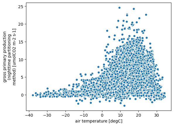
We can also use a similar method to plot a scatterplot of one variable against another one. However, this can take some time to run, therefore reducing the data can be helpful. Here we select every 10th site and take the weekly mean to plot air temperature vs. GPP:

ds_subset = ds.isel(site=slice(None, None, 10))  # take every 10th site for reduced data
ds_subset.resample(time="1W").mean().plot.scatter(x="ta", y="gpp_nt")

<matplotlib.collections.PathCollection at 0x14013d350>